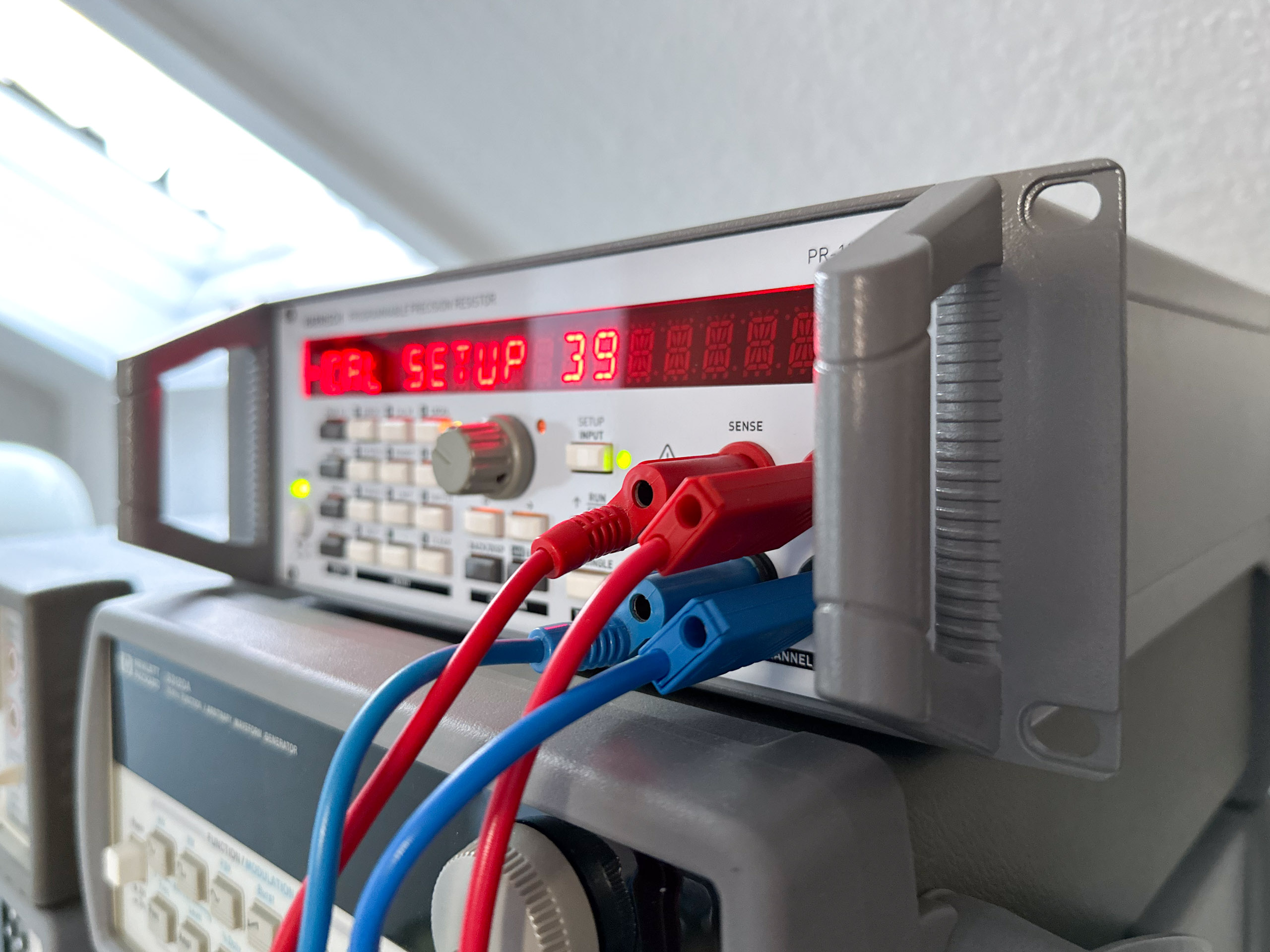
After the modification described in the previous post I let the the “adjustment”/calibration procedure run again. Five days later I repeated the calibration (not the adjustment). As before, all measurements are performed with an Agilent 34401A 6.5 digit multimeter.
Accuracy of the resistance
First up is a diagram that shows the absolute value of the deviation of the measurement value from the setpoint. The tested values are grouped as follows:
- Calibration points: There are 55 calibration points (0, 1, 2, .., 9; 10, 20, .., 90; 100, 200, .., 900; 1k, 2k, .., 9k; 10k, 20k, .., 90k; 100k, 200k, .., 900k). In the diagram, all calibration points are connected via lines for visual purposes only. This does NOT imply that we can estimate the deviation for setpoints between two calibration points by looking at this line.
- Validation points: These are 9 randomly selected values per decade for the upper five decades. All values of the first decade are already included in the calibration points. This results in 45 additional points. Validation points are not connected by a line
The diagram includes curves for the following scenarios:
- UNCAL@4W: The unit is used in its uncalibrated mode, where the user selectable setpoint equals the hardware setpoint. If, for example, the user enters \(130\text{ k}\Omega\), the 6th decade would be in the \(100\text{ k}\Omega\), the 5th decade in the \(30\text{ k}\Omega\) and all lower decades in the shorted position. Also, the display logic ignores the calibration constants and shows \(130.000\text{ k}\Omega\). (The input LED switches to red in order to indicate the uncalibrated mode.) For the diagram shown, the measurement was performed using a four-wire resistance measurement
- 2W: In the calibrated two-wire mode, the unit uses the two-wire calibration constants to optimize the hardware setpoint so that the actual resistance value is as close to the setpoint as possible. The calibration in this scenario is also performed using two-wire measurements
- 4W: In the calibrated four-wire mode, the unit uses the four-wire calibration constants to optimize the hardware setpoint so that the actual resistance value is as close to the setpoint as possible. The calibration in this scenario is also performed using four-wire measurements
There are two curves to asses whether/which specifications can be fulfilled:
- In order to compare the results with the requirements defined in the first post, the diagram shows a curve where the absolute value of the deviation would be equal to \(0.5\% \text{ of value}+ 0.3\text{ }\Omega\)
- A second curve narrows the spec down to \(0.1\% \text{ of value} + 0.15\text{ }\Omega\)
The test setup isn’t perfect either. Three curves characterize the accuracy we can expect from the Agilent 34401A multimeter (absolute value; measured values could deviate in positive as well as negative direction). These are based on a Keysight datasheet (published in USA, July 8, 2022).

There are multiple observations we can make:
- With very high confidence, the absolute deviation is significantly below \(0.5\% + 0.3\text{ }\Omega\), hence I consider the requirement fulfilled
- The randomly selected validation points show deviations that are close to deviations seen for calibration points close by
- The 34401A is not necessarily multiple orders of magnitude more accurate than the resistors used, especially if not calibrated 24h beforehand. So evaluating the absolute accuracy using this setup seems to be a bit difficult
- I adjusted the unit so that it complies with the measurement results of the 34401A as good as possible. The strong improvements seen for higher setpoint values indicate that the algorithm actually does what it is supposed to do: For setpoints \(\ge 50\text{ k}\Omega\) the deviation can be reduced by an order of magnitude or thereabouts. There is no point in trying to adjust the resistance manually, the algorithm takes care of it well enough, when it’s possible to improve something
- Assuming the 34401A measures the resistance perfectly (it doesn’t) the deviation is below \(0.1\% + 0.15\text{ }\Omega\) for all tested setpoints
Accuracy of the calculated resistance value
The second diagram is similar to some extent, but instead of comparing the setpoint with the actual (measured) resistance, now we compare the calculated resistance (estimate based on the calibration values) with the actual (measured) resistance. This answers the question of whether we have to measure the resistance each time we select a value, or whether it’s ok to just look at the unit and trust that the value displayed is the resistance at the input.

Like with the accuracy, for really low resistance values there is some significant deviation* (worst case about 2% for 2W and 1% for 4W at \(1\text{ }\Omega\)). However, the deviation drops really quickly. For resistance values above \(10\text{ }\Omega\) we’re looking at about 0.1% deviation or less, for \(100\text{ }\Omega\) and up at a deviation of about 0.01% or less which I consider irrelevant in almost any situation the unit could be used in. In other words: In most cases the estimate is roughly one order of magnitude more accurate than the accuracy of the resistance. This leads me to the conclusion that the calculated resistance can be relied upon, with certain caveats for really low values (however, those also apply for the accuracy too).
* This deviation could likely be reduced further with a software update that also stores the calibration data for the lowest decade without any compensation for the contact resistance etc. that is only required for higher decades.
More data
| Applied value (\(\Omega\)) | Calculated value (\(\Omega\)) | Indicated value (\(\Omega\)) | Previous indicated value (\(\Omega\)) | Deviation (\(\%\)) | Previous Deviation (\(\%\)) |
|---|---|---|---|---|---|
| 0 | 0.079 | 0.071 | 0.070 | – | |
| 1 | 1.062 | 1.053 | 1.052 | 5.263533333 | 5.2383 |
| 2 | 2.033 | 2.028 | 2.074 | 1.408816667 | 3.7170 |
| 3 | 3.012 | 3.006 | 3.052 | 0.2079 | 1.7271 |
| 4 | 4.033 | 4.026 | 4.073 | 0.662033333 | 1.8132 |
| 5 | 5.012 | 5.005 | 5.050 | 0.09504 | 1.0041 |
| 6 | 6.033 | 6.025 | 6.072 | 0.412716667 | 1.1936 |
| 7 | 7.011 | 7.003 | 7.049 | 0.043942857 | 0.7020 |
| 8 | 8.031 | 8.022 | 8.069 | 0.2806375 | 0.8623 |
| 9 | 9.009 | 9.001 | 9.047 | 0.008366667 | 0.5178 |
| 10 | 10.122 | 10.107 | 10.108 | 1.073303333 | 1.0764 |
| 20 | 20.082 | 20.074 | 20.123 | 0.37111 | 0.6164 |
| 30 | 30.068 | 30.059 | 30.107 | 0.197274444 | 0.3557 |
| 40 | 40.084 | 40.077 | 40.125 | 0.192709167 | 0.3127 |
| 50 | 50.070 | 50.062 | 50.109 | 0.12339 | 0.2172 |
| 60 | 60.080 | 60.072 | 60.120 | 0.120141667 | 0.2001 |
| 70 | 70.065 | 70.057 | 70.103 | 0.08075 | 0.1478 |
| 80 | 80.076 | 80.068 | 80.116 | 0.084922917 | 0.1446 |
| 90 | 90.060 | 90.053 | 90.099 | 0.058452963 | 0.1101 |
| 100 | 100.073 | 100.061 | 100.061 | 0.061116667 | 0.0609 |
| 200 | 200.010 | 200.002 | 200.003 | 0.001085 | 0.0014 |
| 300 | 299.896 | 299.891 | 299.891 | -0.03625 | -0.0363 |
| 400 | 399.859 | 399.860 | 399.860 | -0.0351175 | -0.0351 |
| 500 | 499.744 | 499.747 | 499.748 | -0.050556 | -0.0504 |
| 600 | 599.633 | 599.636 | 599.639 | -0.06065 | -0.0602 |
| 700 | 699.518 | 699.523 | 699.527 | -0.06814619 | -0.0676 |
| 800 | 799.431 | 799.434 | 799.440 | -0.070715417 | -0.0700 |
| 900 | 900.300 | 900.304 | 900.310 | 0.033734444 | 0.0345 |
| 1000 | 1000.200 | 1000.162 | 1000.161 | 0.01622 | 0.0161 |
| 2000 | 2000.383 | 2000.319 | 2000.276 | 0.015946667 | 0.0138 |
| 3000 | 3000.273 | 3000.206 | 3000.136 | 0.006882222 | 0.0045 |
| 4000 | 4000.661 | 4000.679 | 4000.605 | 0.0169725 | 0.0151 |
| 5000 | 5000.539 | 5000.552 | 5000.471 | 0.011046 | 0.0094 |
| 6000 | 6001.060 | 6001.124 | 6001.056 | 0.018730556 | 0.0176 |
| 7000 | 7000.929 | 7000.985 | 6999.094 | 0.014064762 | -0.0129 |
| 8000 | 8001.034 | 8001.093 | 7998.958 | 0.013662083 | -0.0130 |
| 9000 | 9000.900 | 9000.951 | 8999.083 | 0.010567778 | -0.0102 |
| 10000 | 9998.890 | 9998.835 | 9998.949 | -0.011650333 | -0.0105 |
| 20000 | 20000.368 | 20001.168 | 20001.205 | 0.00584 | 0.0060 |
| 30000 | 29999.829 | 29999.140 | 29999.199 | -0.002866667 | -0.0027 |
| 40000 | 40000.393 | 39999.804 | 39998.617 | -0.000489167 | -0.0035 |
| 50000 | 50000.468 | 49999.627 | 49998.765 | -0.000746 | -0.0025 |
| 60000 | 60000.023 | 59999.575 | 59999.367 | -0.000708889 | -0.0011 |
| 70000 | 70000.238 | 70000.223 | 70000.372 | 0.000318095 | 0.0005 |
| 80000 | 79999.625 | 79999.481 | 79999.635 | -0.000648333 | -0.0005 |
| 90000 | 90000.015 | 89999.845 | 90000.060 | -0.000171852 | 0.0001 |
| 100000 | 100000.280 | 99999.540 | 99999.994 | -0.000459667 | 0.0000 |
| 200000 | 200000.086 | 199999.253 | 200001.770 | -0.000373333 | 0.0009 |
| 300000 | 300000.414 | 300000.953 | 300004.140 | 0.000317778 | 0.0014 |
| 400000 | 400000.057 | 400001.630 | 400007.160 | 0.0004075 | 0.0018 |
| 500000 | 499999.939 | 500001.013 | 500009.000 | 0.000202667 | 0.0018 |
| 600000 | 599999.505 | 600003.553 | 600015.190 | 0.000592222 | 0.0025 |
| 700000 | 700000.073 | 700001.357 | 700015.190 | 0.00019381 | 0.0022 |
| 800000 | 799999.583 | 799999.317 | 800017.240 | -8.54167E-05 | 0.0022 |
| 900000 | 899999.680 | 899997.450 | 900018.830 | -0.000283333 | 0.0021 |
Conclusion
With the fairly stable resistors used and also great calibration results I think it’s fair to call it a precision instrument. Hence the label Programmable Precision Resistor on the front panel. That being said: If you’re looking at an accuracy in the ppm range, things like EMF and the isolation material of the binding posts matter. Those effects were not considered.
Also, there are some other topics that could be very interesting like temperature and long term drift (e. g. 30 days, 90 day, 1 year). I don’t have a climate chamber, but running the automated calibration procedure would certainly be an option.