In the last post we selected a resistor network and switch topology that suits the needs of this programmable resistor. Now we will apply simple optimizations that allow an effective and cost-efficient implementation.

Optimizing the bill of material
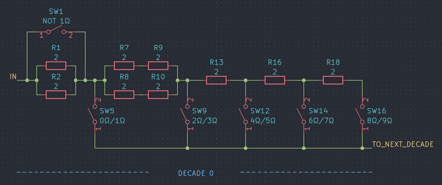
In order to reduce the number of different components the single \(1 \Omega\) is replaced by two parallel \(2 \Omega\) resistors. As a very welcome side effect this doubles the power rating for the setting \(1 \Omega\). This is very helpful, because the lower the selected resistance value of the decade, the fewer resistors the power dissipation is distributed over.
For this very reason it can be very beneficial to increase the power dissipation capabilities of the first two ohm increment as well – otherwise the corresponding resistor would become the bottleneck in regards to power dissipation. We can achieve this by replacing the single \(2\Omega\) resistor by four \(2\Omega\) resistors used in a parallel connection of to series connections. Due to quantity discount, using a total of 9 identical resistors isn’t quite as bad as the number might suggest. Therefore the final design looks like that:

Now the question is: What are the current handling and total power dissipation capabilities and the maximum allowable voltage for both an individual decade and the programmable resistor decade, as the answer may vary for different resistance settings? Well, we will discuss that in the next posts.