Now that we have a calibrated programmable resistance decade, we can try to make the programmable decade resistor more accuracte – for higher resistance values. Actually, the idea behind that is trivial.
I’d like to start with an example in which we set a resistance value of \(R_{set} = 100.000\text{ k}\Omega\). (Let’s not worry about temp drift, contact resistance etc.) In my case all resistors have a specified tolerance of \(0.1\%\). So we’d expect a resistance somewhere in the range of
$$99.900\text{ k}\Omega \leq R_{meas} \leq 100.100\text{ k}\Omega$$
Let’s assume we estimated a resistance of \(R_{est} = 99.952\text{ k}\Omega\) based on the calibration values. Now it’s pretty obvious that we can use the lower two decades to add some additional resistance – \(40\text{ }\Omega\) from the second decade and \(8\text{ }\Omega\) from the first decade should do the trick. And with \(0.1\%\) resistors we know that we’ll achieve a value very, very close to \(48\text{ }\Omega\). The actual setpoint that I will call the hardware setpoint has now become (\(R_{hwset} = 100.048\text{ k}\Omega\)).
But care must be taken: In a more generalized sense the lower decades deviate from the theoretical value as well due to their tolerance. Had I chosen an estimated resistance \(R_{est} > 100.000\text{ k}\Omega\), it would have been not only a little more paperwork, but we would have ended up with a hardware setpoint below \(100.000\text{ k}\Omega\), e. g. \(R_{hwset} = 99,910\text{ }\Omega\). Now it’s easy to see that not only the highest decade might introduce a relevant error, but also multiple lower decades: Decade 4 (i. e. the fifth decade) could deviate by \(90\text{ }\Omega\), decade 3 by \(9\text{ }\Omega\) and decade 2 by \(0.9\text{ }\Omega\).
A simple approach for calculating the optimal hardware setpoint would be to use brute force and set up a look-up table that keeps the hardware setpoint in memory for any given setpoint. Certainly, such a look-up table can be accessed very quickly. But even on a computer a completely non-optimized approach for generating the look-up table can be rather time consuming. Whereas memory usage isn’t a concern in that case, with microcontrollers this would be a completly different story: Good luck finding a (cheap) microcontroller with >4 MByte of Flash memory (1M datapoints with 4 Byte each if we are talking 6 decades). Also, the look-up table would have to be re-calculated whenever the programmable decade resistor is calibrated and this would take really long on a microcontroller.
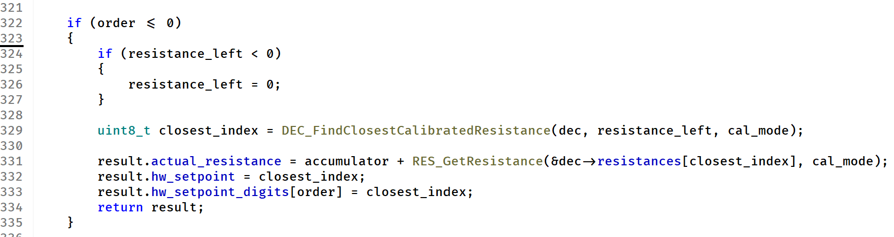
In many cases we’d get away with such a lazy approach, but not this time. We need an algorithm that uses the current calibration values as an input and is able to narrow down the solution space in a way that allows for calculation in real time: Branch and bound.
The obvious idea is to start the selection process at the highest decade. In our previous example we wanted to achieve \(R_{set} = 100.000\text{ k}\Omega\). With a tolerance of the resistors of \(0.1\%\) we can be sure that decade 5 has to be either a “1” (\(100.000\text{ k}\Omega\)) or a “0” (\(0\Omega\)). If option “1” results in a resistance value greater than the setpoint, then we don’t have to try to add any more resistance – this already would be the best we can do with this option. If it is below, then we apply the algorithm again, but now limited to the 5 lower decades and with the remaining Ohms as the new target. After that we repeat for option “0” and ultimately figure out who the winner was.
A few hints and notes:
- The algorithm described can be implemented fairly easily with recursion. A good thing: The recursion depth is limited by the (fixed) number of decades, so that shouldn’t become a problem if done properly
- It’s the resistors’ tolerances that decides which options have to be checked
- Eliminate as many of the options as required to reach the performance goals while factoring in the constraints imposed by the tolerances of the resistors
- For obvious reasons the accuracy of the calibration directly impacts the results of this approach
- The algorithm will achieve benefits for larger resistance values only
As for the calibration procedure, I plan to do an evaluation of this optimization in a future post of this series.
Leave a Reply